Category: Open Source
Java 26: 10 JEPs Explained for Developers
Java 26 landed on 17 March 2026, right on schedule as Oracle’s relentless six month cadence demands. As the first non-LTS release since Java 25, it ships ten JDK Enhancement Proposals, or JEPs. A JEP is the formal unit of change in the Java platform: a numbered design document authored by engineers from Oracle, the […]
Read more →Shift+Click Dock Icon to Cycle App Windows on macOS
If you run multiple Chrome profiles or keep several windows open per app, switching between them on macOS becomes irritating fast. Clicking the Dock icon only brings the app forward. Clicking it again does nothing useful. So you right click, scan the window list, and manually choose the one you want. It breaks flow and […]
Read more →WordPress Site Crashed After Plugin Update: Fix It Fast
You updated a plugin five minutes ago. Maybe it was a security patch. Maybe you were trying a new caching layer. You clicked “Update Now,” saw the progress bar fill, got the green tick, and moved on with your day. Now the site is down. Not partially down. Not slow. Gone. A blank white page. […]
Read more →How to Publish Code on GitHub: Automate It Right
GitHub is not just a code hosting platform. It is your public engineering ledger. It shows how you think, how you structure problems, how you document tradeoffs, and how you ship. If you build software and it never lands on GitHub, as far as the wider technical world is concerned, it does not exist. This […]
Read more →WordPress Plugin Upgrades: Fix Stale File Issues
Most WordPress plugin developers eventually hit the same invisible wall: you ship an update, everything looks correct in the zip, the version number changes, the code is cleaner, and yet users report that the old JavaScript is still running. You check the file. It is updated. They clear cache. Still broken. Here is the uncomfortable […]
Read more →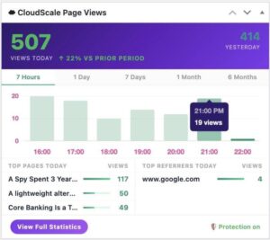
CloudScale PageViews: Fix WordPress Analytics Behind Cloudflare
If you run a WordPress site behind Cloudflare, your page view numbers are lying to you. Jetpack Stats, WP Statistics, Post Views Counter and nearly every other WordPress analytics plugin share the same fatal flaw: they count views on the server. When Cloudflare serves a cached HTML page (which is the entire point of using […]
Read more →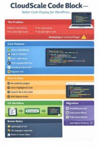
CloudScale Code Block Plugin: Syntax Highlighting for WordPress
If you run a technical blog on WordPress, you know the pain. You paste a markdown article with fenced code blocks, Gutenberg creates bland core/code blocks with no syntax highlighting, no copy button, no dark mode. You end up wrestling with third party plugins that haven’t been updated in years or manually formatting every code […]
Read more →
WordPress Database & Media Cleanup Plugin: Free Guide
If you run a WordPress site for any length of time, the database quietly fills with junk. Post revisions stack up every time you hit Save. Drafts you abandoned years ago sit there. Spam comments accumulate. Transients expire but never get deleted. Orphaned metadata from plugins you uninstalled months ago quietly occupies table rows nobody […]
Read more →What Is Minification and How to Test If It Works
1. What is Minification Minification is the process of removing everything from source code that a browser does not need to execute it. This includes whitespace, line breaks, comments, and long variable names. The resulting file is functionally identical to the original but significantly smaller. A CSS file written for human readability might look like […]
Read more →
CloudScale Free WordPress Backup & Restore Plugin Guide
I’ve been running this blog on WordPress for years, and the backup situation has always quietly bothered me. The popular backup plugins either charge a monthly fee, cap you on storage, phone home to an external service, or do all three. I wanted something simple: a plugin that makes a zip file of my site, […]
Read more →