Author: Andrew Baker

Management vs Leadership: Why Promoting Managers Fails
Management and leadership sound so similar that they are often used interchangeably. True, they are both a sport. But details matter when you want to win. Nowhere is this more visible than in financial services. Banks today do not compete inside a known, stable competitive set. The threat landscape runs from a two-person fintech with […]
Read more →
Why Bolting AI onto Existing Org Structures Always Fails
There is an old urban legend, immortalised as one of the original Darwin Award nominations, about a man who bolted a JATO unit to a 1967 Chevrolet Impala. JATO stands for Jet Assisted Take Off. It is a solid fuel rocket designed to give heavy military transport aircraft the extra thrust they need to leave […]
Read more →
How Product Team Structures Inflate Engineer Performance Ratings
There is a product team performance bias hiding in plain sight inside every organisation that has moved to product aligned engineering, except that it does not show up as a number on a dashboard, a flag in a talent calibration session, or a red line in an engagement survey. It accumulates quietly, year on year, […]
Read more →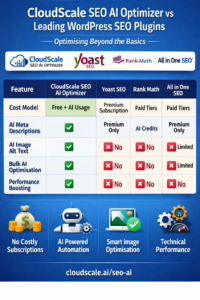
Free AI WordPress SEO Plugin: CloudScale vs Yoast & Rank Math
1. Introduction Download the plugin here: https://wordpress.org/plugins/cloudscale-seo-ai-optimizer/ S3 download (updated frequently): https://andrewninjawordpress.s3.af-south-1.amazonaws.com/cloudscale-seo-ai-optimizer.zip For more than a decade the WordPress SEO landscape has been dominated by a small group of plugins. Yoast SEO, Rank Math, and All in One SEO have collectively powered millions of sites and shaped how authors think about optimisation. These plugins are […]
Read more →SEO and AEO Page Audit Script: A Technical Guide
Search engines no longer operate alone. Your content is now consumed byGoogle, Bing, Perplexity, ChatGPT, Claude, Gemini, and dozens of otherAI driven systems that crawl the web and extract answers. Classic SEO focuses on ranking. Modern discovery also requires AEO (Answer Engine Optimization) which focuses on being understood and extracted by AI systems. A marketing […]
Read more →
Capitec Pulse: The Engineering Behind Real-Time AI at Scale
By Andrew Baker, Chief Information Officer, Capitec Bank The Engineering Behind Capitec Pulse 1. Introduction I have had lots of questions about how we are “reading our clients minds”. This is a great question, but the answer is quite complex – so I decided to blog it. The article below really focuses on the heavy […]
Read more →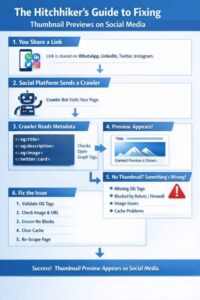
Fix Thumbnail Previews on WhatsApp, LinkedIn & X (Guide)
When you share a link on WhatsApp, LinkedIn, X, or Instagram and nothing appears except a bare URL, it feels broken in a way that is surprisingly hard to diagnose. The page loads fine in a browser, the image exists, the og:image tag is there, yet the preview is blank. This post gives you a […]
Read more →
Predict EBS and RDS IOPS Saturation Before It Breaks
Andrew Baker | March 2026 Companion article to: https://andrewbaker.ninja/2026/03/01/aws-iops-mismatch-fix-the-hidden-double-ceiling-bug/ Last week I published a script that scans your AWS estate and finds every EBS volume and RDS instance where your provisioned storage IOPS exceed what the compute instance can actually consume. That problem, the structural mismatch between storage ceiling and instance ceiling, is important and […]
Read more →Chrome MCP for Claude Desktop: Install in One Script
If you have ever sat there manually clicking through a UI, copying error messages, and pasting them into Claude just to get help debugging something, I have good news. There is a better way. Chrome MCP gives Claude Desktop direct access to your Chrome browser, allowing it to read the page, inspect the DOM, execute […]
Read more →Shift+Click Dock Icon to Cycle App Windows on macOS
If you run multiple Chrome profiles or keep several windows open per app, switching between them on macOS becomes irritating fast. Clicking the Dock icon only brings the app forward. Clicking it again does nothing useful. So you right click, scan the window list, and manually choose the one you want. It breaks flow and […]
Read more →