Category: Public Cloud

I Have Two Outlooks on a NASA Spacecraft and Neither Works
1. Ground Control to Major Redmond In early April 2026, four astronauts aboard the Orion spacecraft radioed Mission Control. They were travelling at over four thousand miles per hour, more than thirty thousand miles from Earth, on NASA’s first crewed lunar mission in more than fifty years. The hardware that got them there represents the […]
Read more →
Why Multicloud Is Not a Cloud Resilience Strategy
There is a particular kind of nonsense that circulates in enterprise technology conversations, the kind that sounds like wisdom because it wears the clothes of prudence. Multicloud architecture as a cloud resilience strategy is that nonsense. It has the shape of risk management and the substance of a comfort blanket, and the industry has spent […]
Read more →
Predict EBS and RDS IOPS Saturation Before It Breaks
Andrew Baker | March 2026 Companion article to: https://andrewbaker.ninja/2026/03/01/aws-iops-mismatch-fix-the-hidden-double-ceiling-bug/ Last week I published a script that scans your AWS estate and finds every EBS volume and RDS instance where your provisioned storage IOPS exceed what the compute instance can actually consume. That problem, the structural mismatch between storage ceiling and instance ceiling, is important and […]
Read more →AWS IOPS Mismatch: Fix the Hidden Double Ceiling Bug
Andrew Baker, Chief Information Officer at Capitec Bank There is a class of AWS architecture mistake that is genuinely difficult to see. It does not appear in your cost explorer as an obvious line item. It does not trigger a CloudWatch alarm. It does not show up in a well architected review unless the reviewer […]
Read more →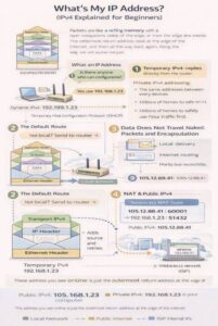
What Is My IP Address? IPv4 Explained for Beginners
Firstly, let me acknowledge that there are lots of these kinds of posts on the internet. But the reason why i wrote this blog is that I wanted to force myself to consolidate the various articles I have read and my learnt knowledge in this space. I will probably update this article several times and […]
Read more →WordPress on AWS Graviton: Deploy & Migrate in Minutes
Running WordPress on ARM-based Graviton instances delivers up to 40% better price-performance compared to x86 equivalents. This guide provides production-ready scripts to deploy an optimised WordPress stack in minutes, plus everything you need to migrate your existing site. Why Graviton for WordPress? Graviton3 processors deliver: The t4g.small instance (2 vCPU, 2GB RAM) at ~$12/month handles […]
Read more →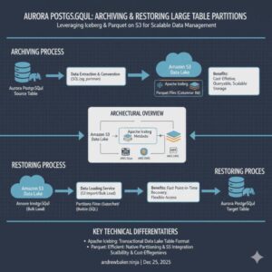
Aurora PostgreSQL: Archive Partitions to S3 Iceberg & Parquet
A Complete Guide to Archiving, Restoring, and Querying Large Table Partitions When dealing with multi-terabyte tables in Aurora PostgreSQL, keeping historical partitions online becomes increasingly expensive and operationally burdensome. This guide presents a complete solution for archiving partitions to S3 in Iceberg/Parquet format, restoring them when needed, and querying archived data directly via a Spring […]
Read more →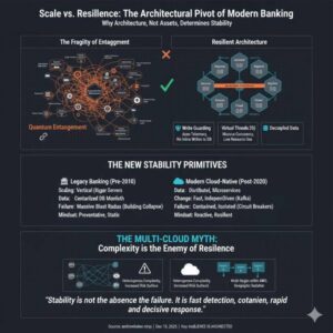
Why Bank Architecture Determines Resilience More Than Size
1. Size Was Once Mistaken for Stability For most of modern banking history, stability was assumed to increase with size. The thinking was the bigger you are, the more you should care, the more resources you can apply to problems. Larger banks had more capital, more infrastructure, and more people. In a pre-cloud world, this […]
Read more →PostgreSQL Prepared Statements: Fix Plan Caching Memory Issues
Prepared statements are one of PostgreSQL’s most powerful features for query optimization. By parsing and planning queries once, then reusing those plans for subsequent executions, they can dramatically improve performance. But this optimization comes with a hidden danger: sometimes caching the same plan for every execution can lead to catastrophic memory exhaustion and performance degradation. […]
Read more →AWS CLI Setup on Mac: Install and Configure in Minutes
You can absolutely get the following from the AWS help pages; but this is the lazy way to get everything you need for a simple single account setup. Run the two commands below to drop the package on your Mac. Then check the versions you have installed: Next you need to setup your environment. Note: […]
Read more →