Category: Linux
Enable Claude Desktop To Run Bash MCP : Fully Scripted Installation
Andrew Baker | 01 Mar 2026 | andrewbaker.ninja You want one script that does everything. No digging around in settings. No manually editing JSON. No clicking Developer, Edit Config. Just run it once and Claude Desktop can execute bash commands through an MCP server. This guide gives you exactly that. 1. Why You Would Want […]
Read more →
A Spy Spent 3 Years Planting a Backdoor to Bring the Internet Down. One Person Noticed
On a quiet Friday evening in late March 2024, a Microsoft engineer named Andres Freund was running some routine benchmarks on his Debian development box when he noticed something strange. SSH logins were taking about 500 milliseconds longer than they should have. Failed login attempts from automated bots were chewing through an unusual amount of […]
Read more →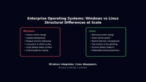
The 10 Biggest Differences Between Windows Server and Linux for Enterprises
Enterprise operating systems for servers, are not chosen because they are liked. They are chosen because they survive stress. At scale, an operating system stops being a piece of software and becomes an amplifier of either discipline or entropy. Every abstraction, compatibility promise, and hidden convenience eventually expresses itself under load, during failure, or in […]
Read more →
Redis vs Valkey: A Deep Dive for Enterprise Architects
The in memory data store landscape fractured in March 2024 when Redis Inc abandoned its BSD 3-clause licence in favour of the dual RSALv2/SSPLv1 model. The community response was swift and surgical: Valkey emerged as a Linux Foundation backed fork, supported by AWS, Google Cloud, Oracle, Alibaba, Tencent, and Ericsson. Eighteen months later, both projects […]
Read more →Understanding and Detecting CVE-2024-3094: The React2Shell SSH Backdoor
Executive Summary CVE-2024-3094 represents one of the most sophisticated supply chain attacks in recent history. Discovered in March 2024, this vulnerability embedded a backdoor into XZ Utils versions 5.6.0 and 5.6.1, allowing attackers to compromise SSH authentication on Linux systems. With a CVSS score of 10.0 (Critical), this attack demonstrates the extreme risks inherent in […]
Read more →Deep Dive: AWS NLB Sticky Sessions (stickiness) Setup, Behavior, and Hidden Pitfalls
When you deploy applications behind a Network Load Balancer (NLB) in AWS, you usually expect perfect traffic distribution, fast, fair, and stateless.But what if your backend holds stateful sessions, like in-memory login sessions, caching, or WebSocket connections and you need a given client to keep hitting the same target every time? That’s where NLB sticky […]
Read more →Mac OSX : Tracing which network interface will be used to route traffic to an IP/DNS address
If you have multiple connections on your device (and maybe you have a zero trust client installed); how do you find out which network interface on your device will be used to route the traffic? Below is a route get request for googles DNS service: If you have multiple interfaces enabled, then the first item […]
Read more →Macbook Tip: iTerm2 clearing your scroll back history
I frequently forget this command shortcut, so this post is simply because I am lazy. To clear your history in iTerm press Command + K. Control + L only clears the screen, so as soon as you run the next command you will see the scroll back again. If you want to view your command […]
Read more →Macbook: Querying DNS using the Host Command
1. Find a list of IP addresses linked to a domain To find the IP address for a particular domain, simply pass the target domain name as an argument after the host command. For a comprehensive lookup using the verbose mode, use -a or -v flag option. The -a option is used to find all Domain records and Zone […]
Read more →Macbook: Changing prompt $ information in the mac terminal window
When you open terminal you will see that it defaults the information that you see on the prompt, which can use up quite a bit of the screen real estate. Customize the zsh Prompt in Terminal Typically, the default zsh prompt carries information like the username, machine name, and location starting in the user’s home […]
Read more →