AWS, Cloud & Database Architecture
23 views
Banking-grade AWS deployments, multi-cloud trade-offs, and database design at scale. The architectural decisions that prevent 3am incidents.

The Hitchhiker’s Guide to Production Outage Triage with Amazon Bedrock
Andrew Baker — andrewbaker.ninja — 13 June 2026 How to use a large language model inside your own AWS account to interrogate your infrastructure while it is on fire So your production environment is throwing errors at 2 AM, your on-call engineer is staring at a wall of CloudWatch noise, and someone in the incident […]
Read more →
AWS IOPS Mismatch: Fix the Hidden Double Ceiling Bug
Andrew Baker, Chief Information Officer at Capitec Bank There is a class of AWS architecture mistake that is genuinely difficult to see. It does not appear in your cost explorer as an obvious line item. It does not trigger a CloudWatch alarm. It does not show up in a well architected review unless the reviewer […]
Read more →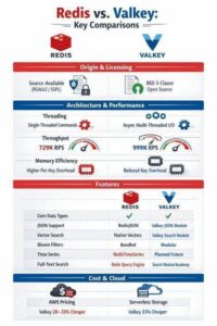
Redis vs Valkey: Enterprise Architecture Guide 2025
The in memory data store landscape fractured in March 2024 when Redis Inc abandoned its BSD 3-clause licence in favour of the dual RSALv2/SSPLv1 model. The community response was swift and surgical: Valkey emerged as a Linux Foundation backed fork, supported by AWS, Google Cloud, Oracle, Alibaba, Tencent, and Ericsson. Eighteen months later, both projects […]
Read more →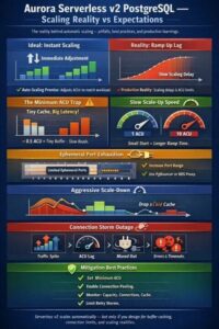
Aurora Serverless v2 PostgreSQL: Production Scaling Guide
Aurora Serverless v2 promises the dream of a database that automatically scales to meet demand, freeing engineering teams from capacity planning. The reality is considerably more nuanced. After running Serverless v2 PostgreSQL clusters under production workloads, I have encountered enough sharp edges to fill a blog post. This is that post. The topics covered here […]
Read more →
PostgreSQL Vacuum Optimization for Large Tables: Deep Dive
When managing large PostgreSQL tables with frequent updates, vacuum operations become critical for maintaining database health and performance. In this comprehensive guide, we’ll explore vacuum optimization techniques, dive deep into the pg_repack extension, and provide hands-on examples you can run in your own environment. 1. Understanding the Problem PostgreSQL uses Multi-Version Concurrency Control (MVCC) to […]
Read more →
Amazon Aurora DSQL: Performance, Limits & Architecture
1. Executive Summary Amazon Aurora DSQL represents AWS’s ambitious entry into the distributed SQL database market, announced at re:Invent 2024. It’s a serverless, distributed SQL database featuring active active high availability and PostgreSQL compatibility. While the service offers impressive architectural innovations including 99.99% single region and 99.999% multi region availability, but it comes with significant […]
Read more →
I Have Two Outlooks on a NASA Spacecraft and Neither Works
1. Ground Control to Major Redmond In early April 2026, four astronauts aboard the Orion spacecraft radioed Mission Control. They were travelling at over four thousand miles per hour, more than thirty thousand miles from Earth, on NASA’s first crewed lunar mission in more than fifty years. The hardware that got them there represents the […]
Read more →
Rubrik Architecture: Why Restore, Not Backup, Is the Product
1. Backups Should Be Boring (and That Is the Point) Backups are boring. They should be boring. A backup system that generates excitement is usually signalling failure. The only time backups become interesting is when they are missing, and that interest level is lethal. Emergency bridges. Frozen change windows. Executive escalation. Media briefings. Regulatory apology […]
Read more →
Why Multicloud Is Not a Cloud Resilience Strategy
There is a particular kind of nonsense that circulates in enterprise technology conversations, the kind that sounds like wisdom because it wears the clothes of prudence. Multicloud architecture as a cloud resilience strategy is that nonsense. It has the shape of risk management and the substance of a comfort blanket, and the industry has spent […]
Read more →Predict EBS and RDS IOPS Saturation Before It Breaks
Andrew Baker | March 2026 Companion article to: https://andrewbaker.ninja/2026/03/01/aws-iops-mismatch-fix-the-hidden-double-ceiling-bug/ Last week I published a script that scans your AWS estate and finds every EBS volume and RDS instance where your provisioned storage IOPS exceed what the compute instance can actually consume. That problem, the structural mismatch between storage ceiling and instance ceiling, is important and […]
Read more →
AWS Security Group Hardening Using VPC Flow Log Analysis: Introducing sg-tightener
Andrew Baker, Group CIO, Capitec Bank Most enterprises did not move to AWS. They extended into it. The datacenter did not go away. The VPN did not go away. The network team provisioned the Direct Connect, someone wrote a security group rule permitting the entire datacenter subnet, and that rule has been sitting there ever […]
Read more →
AWS NLB Sticky Sessions: Setup, Behavior & Pitfalls
When you deploy applications behind a Network Load Balancer (NLB) in AWS, you usually expect perfect traffic distribution, fast, fair, and stateless.But what if your backend holds stateful sessions, like in-memory login sessions, caching, or WebSocket connections and you need a given client to keep hitting the same target every time? That’s where NLB sticky […]
Read more →