Author: Andrew Baker
Keep Your Mac Awake While Claude Code Works
If you run Claude Code in its default local mode, your Mac will happily fall asleep mid-task, killing the session and whatever was being built. The fix is simple, but it is worth knowing about before it bites you. 1. The quickest solution: caffeinate macOS ships with a utility called caffeinate that prevents sleep for […]
Read more →
Lock It Down: The Complete Guide to Securing Your WhatsApp
Your WhatsApp account is not just a chat app. It is your identity, your contacts, your banking OTPs, your family photos, and your most private conversations. When criminals take it over, they use it immediately to impersonate you and defraud everyone you know. This guide walks through every meaningful control available to you, explains what […]
Read more →Migrating a Pi 5 WordPress Stack from SD Card to NVMe
I run a full WordPress stack on a Raspberry Pi 5 sitting on my desk: MariaDB, PHP-FPM, Nginx, and Redis, all inside Docker containers, served publicly through a Cloudflare tunnel. After fitting an NVMe SSD via the Pi 5 HAT+, the obvious next step was getting Docker off the SD card entirely. The SD card […]
Read more →
I Have Two Outlooks on a NASA Spacecraft and Neither Works
1. Ground Control to Major Redmond In early April 2026, four astronauts aboard the Orion spacecraft radioed Mission Control. They were travelling at over four thousand miles per hour, more than thirty thousand miles from Earth, on NASA’s first crewed lunar mission in more than fifty years. The hardware that got them there represents the […]
Read more →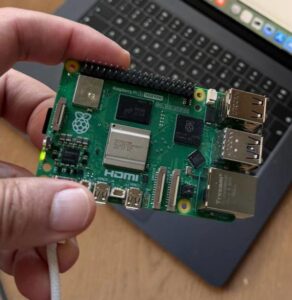
EC2 to Raspberry Pi WordPress Migration: Full Guide
How I moved andrewbaker.ninja off AWS, saved hundreds of dollars a year, and ended up with better security in the process. Running a personal site on AWS is completely reasonable when you are starting out. The tooling is mature, the reliability is excellent, and you can spin up a new instance in seconds. But somewhere […]
Read more →Fix Raspberry Pi Boot Failures: SD to NVMe in 5 Steps
A real-world guide to making your Pi bulletproof, from SD card corruption to NVMe migration I learned this lesson the hard way. My Raspberry Pi 5 was happily serving a production WordPress site when I rebooted it. Two minutes later there was no SSH, no site, just a solid red light staring back at me. […]
Read more →Claude Code Remote Control & Computer Use: 2026 Guide
There is a moment when a tool stops being something you use and becomes something that works for you. That moment, for Claude Code, arrived in early 2026. What began as a terminal-based AI coding assistant has evolved, in the span of a few months, into a platform capable of operating your machine, continuing its […]
Read more →Appium macOS Desktop App Testing: Setup & First Test
Automating native Mac applications with Appium and Claude Code 1. What Appium Actually Is (and Why It Matters for Desktop) Most engineers encounter Appium in a mobile context, but it has always supported native desktop application testing on macOS through its mac2 driver, and this is genuinely useful territory that gets far less attention than […]
Read more →
Why Multicloud Is Not a Cloud Resilience Strategy
There is a particular kind of nonsense that circulates in enterprise technology conversations, the kind that sounds like wisdom because it wears the clothes of prudence. Multicloud architecture as a cloud resilience strategy is that nonsense. It has the shape of risk management and the substance of a comfort blanket, and the industry has spent […]
Read more →
Why We Industrialised the Leadership Vacuum
How we built a global machine to produce administrators, handed them leadership titles, and convinced ourselves that was enough We have built business schools, certification programmes, corporate development curricula and entire consulting industries around the premise that leadership can be systematised, credentialled and scaled. We have invested billions in the proposition. And the returns are […]
Read more →